Table of Contents
Introduction
Where were you when you first heard about the Central Limit Theorem (CLT)?
If you are like me, you heard of the CLT in the classroom as a justification for the assumption of Gaussian noise in the RF environment. The CLT states that the summation of independent random variables (RV) approaches a Gaussian distribution with an increasing number of random variables.
The CLT is convenient in simplifying mathematics, but when and how should it be used? Under what circumstances is it valid?
Let’s take a brief look at how well three different random variables follow the CLT.
More blog posts on DSP Math:
Uniform Random Variable
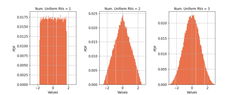
Let us start with a simple case, a uniform random variable on [-1, +1]. Figure 1 shows the estimated probability density function (PDF) for a uniform RVs, the summation of two uniform RVs, and three uniform RVs. In each case the PDF is normalized to have unit variance.
With only two RVs the PDF is triangular in shape and is approaching a Gaussian distribution, and at only three RVs the CLT has taken effect and the distribution is indistinguishable from a Gaussian distribution. The continuous nature of the underlying distribution allows for much faster convergence of the CLT.
Discrete Random Variable
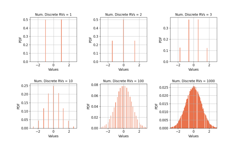
Consider a discrete random variable which approximates BPSK symbols, {-1, +1}. Figure 2 shows that many more RVs are needed to approximate a Gaussian distribution. The triangular distribution be seen at 10 RVs, an outline of a Gaussian distribution can be seen at 100 RVs, but it takes 1000 RVs for Gaussian approximation to be valid. The discrete nature of the distribution requires substantially more RVs for the CLT to apply than the continuous uniform distribution.
Filtered BPSK Symbols
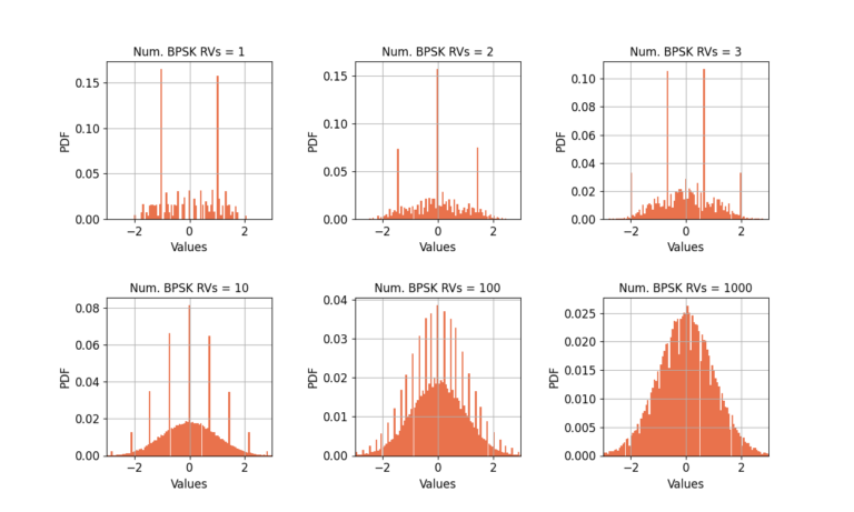
Let’s take it one step further: filtered BPSK symbols with a random center frequency offset (CFO). Figure 3 shows the distribution has elements from both a continuous and discrete distributions. The discrete terms dominate the distribution for a small number of RVs but comes to approximate the Gaussian better as the number increases.
Conclusion
The CLT is a useful tool in simplifying some distributions to a Gaussian approximation but how quickly it converges depends on the underlying distributions as well as the number of random variables in the summation. Be careful to avoid applying it to a situation in which the CLT may not apply or the approximation may not as good as desired.
More blog posts on DSP Math:

