Table of Contents
Introduction
The half band filter (HBF) is an incredibly efficient filtering structure when designed correctly! In this blog I will discuss how to design half band filter weights with the NumPy function remez(), how to select the parameters to maximize the efficiency, and how a folded FIR filter structure can increase the efficiency further.
See other posts in the half band filter series:
Half Band Filter Background
The HBF is fast! For a HBF with an odd filter length N,
- every other weight is 0 (leads to
 multiplies per input sample),
 - can be folded due to even symmetry (N/4 multiplies per input sample) [lyons2011, p.493, p.702],
- can be reduced to N/8 multiples per input sample (!!!) using a polyphase structure [harris2021, p.221].
Not only is the HBF efficient, it has a ton of applications including:
- Efficient filtering [harris2021, p.107],
- Large sample rate change [harris2021, p.234],
- Logarithmic Frequency Processing (Wavelet Transforms) [vaidyanathan1993, p.491],
- Hilbert Transform [carrick2011],
- Perfect Reconstruction and Quadrature Mirror Filter (QMF) banks [harris2021, p.110].
Designing HBF Weights with Remez
Eagle-eyed readers might recognize that the example LPF filter from this blog was a half band filter although the design will be covered again in this blog post.
The cut-off frequency for a half-band filter is at a quarter of the sampling rate ![]() or in normalized units
or in normalized units ![]() . The code to design an example half band filter is given below:
. The code to design an example half band filter is given below:
filterLength = 21
cutoff = 0.25
transBand = 0.1
fPass = cutoff - (transBand/2)
fStop = cutoff + (transBand/2)
fVec = [0, fPass, fStop, 0.5]
aVec = [1, 0]
HBFWeights = scipy.signal.remez(filterLength,fVec,aVec)
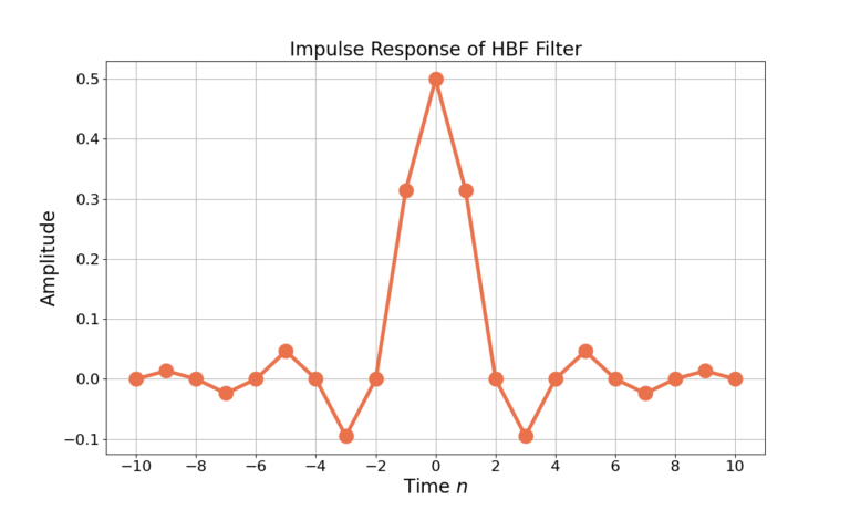
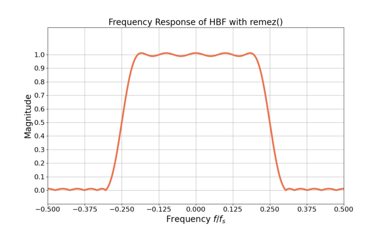
Figure 1 gives the impulse response for the length N=21 filter and the frequency response in Figure 2. Notice from Figure 2 that the magnitude is 0.5 which in log units is ![]() at frequency
at frequency ![]() .
.
Odd Length Half Band Filter
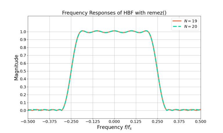
The filter length N=21 was assumed for Figure 1. What happens for other values of filter length N? The impulse for the same HBF with filter length N=19 is given in Figure 3 and it’s frequency response in Figure 4.
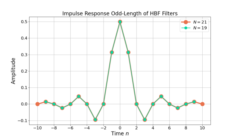
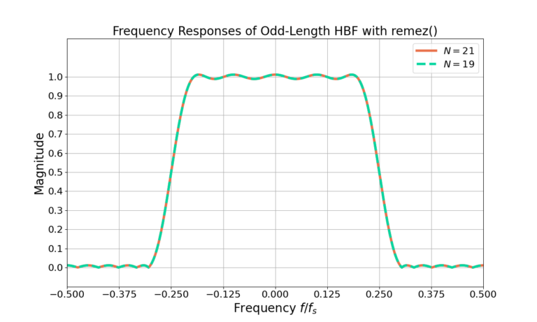
Notice from Figure 3 that although the second filter N=19 is shorter by 2 weights it still has the same linear magnitude frequency response as the N=21 filter in Figure 4. Why?
From Figure 3 it can be seen that the filter weights at n=-10 and n=10 are close to zero. Figure 5 zooms into the filter weights and shows that the even filter weights, with the exception of n=0, are all effectively zero
(1) ![]()
The Remez design algorithm may not force them to zero exactly but can be set that way by a couple of lines of code.
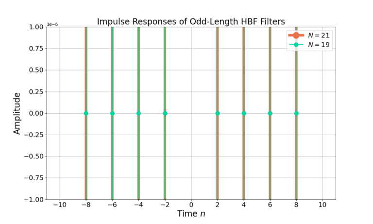
Because the filter weights at n=-10 and n=10 are zero they do not contribute anything to the frequency response and thus are wasted computation. Odd length filters should be designed to have filter lengths
(2) ![]()
where % is the modulo operator. For N=21,
(3) ![]()
which is not desirable for a HBF however for N=19
(4) ![]()
which is an appropriate filter length.
Having zero-weight weights is computationally efficient if implemented correctly. Multiplying by zero always results in zero therefore for filter length N an odd-length HBF can require ![]() multiplies to implement the filter.
multiplies to implement the filter.
Even Length Half Band Filter
What happens when an even length half band filter is designed? Figure 6 gives the impulse response of an even length N=20 half band filter and its frequency response in Figure 7.
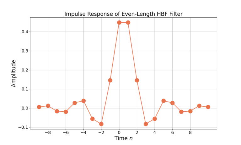
Even length HBF filters do not possess even-symmetry in time (ironic?) and even time index weights are non-zero. The lack of even-symmetry in time will introduce a 1/2 sample delay at the output of the filter and the non-zero weights will require a full N multiplies to implement as compared to ![]() for an odd-length filter. In general an odd-length HBF is a better choice than an even length filter unless there are extenuating circumstances otherwise.
for an odd-length filter. In general an odd-length HBF is a better choice than an even length filter unless there are extenuating circumstances otherwise.
Folding the Half Band Filter Weights
Notice from Figure 3 that the filter weights are even symmetric across n=0 such that
(5) ![]()
An even-symmetric filter can be “folded” so that only one multiplication is done for each unique filter weight. Figure 8 is the block diagram of a generic length N=7 FIR filter, Figure 9 is after the zero-weight have been removed and Figure 10 is the folded implementation of a HBF filter.
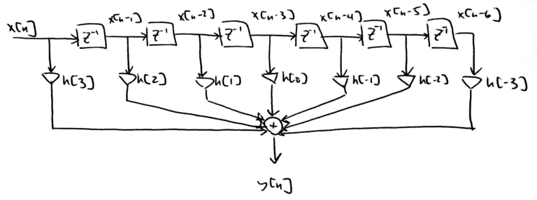

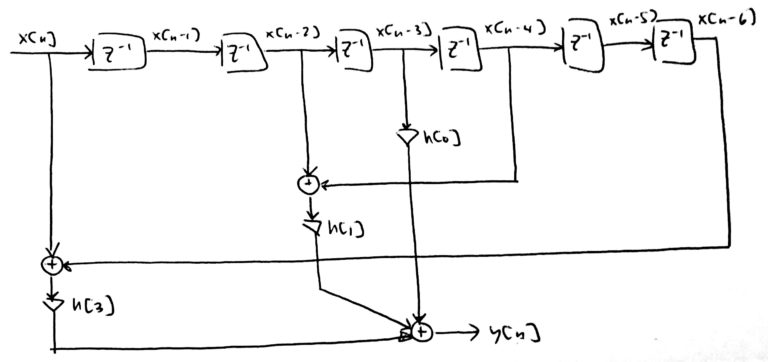
For a length N=7 filter the filter output is
(6) ![]()
which can be expanded to
(7) ![]()
Note that (7) has time-reversed the input signal x[n] for clarity in the math, where as Figure 8 – Figure 10 have time-reversed the filter weights h[n] for graphical clarity. Both representations are valid although Figure 8 – Figure 10 is how the filtering would be implemented in a real world system.
From (1) the zero-weights of h[n] at even indices except for n=0 can be removed from the summation,
(8) ![]()
which reduces the computations from the filter length N=7 to now 5 multiplies. Furthermore due to (5) a pre-addition can be performed to reduce multiplications. For example ![]() therefore
therefore
(9) ![]()
The filter output (8) can be further simplified to
(10) ![Rendered by QuickLaTeX.com \begin{equation*}\begin{split}y[n] & = h[3] (x[-3-n] + x[3-n]) \\& + h[1] ( x[-1-n] + x[1-n]) \\& + x[-n]h[0].\end{split}\end{equation*}](https://www.wavewalkerdsp.com/wp-content/ql-cache/quicklatex.com-3990e7ddcf155546ab628ca788315e2a_l3.png)
From (10) the multiplications have been reduced from N=7 to 3!
Conclusion
The half band filter is an effective tool to have in your kit as it’s computationally efficient and broadly applicable. The HBF is a great foundation understanding more advanced concepts such as the Hilbert transform, performing large sample rate change and near perfect reconstruction filter banks.
Have you seen the other posts on the half band filter?
![A BPSK signal s[n], real Gaussian noise w[n], and the received signal x[n] = s[n] + w[n] for SNR = 20 dB](https://www.wavewalkerdsp.com/wp-content/uploads/wordpress-popular-posts/15621-featured-125x100.png)
![Figure 3: The complex sinusoid e(j2 pi (2/4) n) only contains energy at X[2].](https://www.wavewalkerdsp.com/wp-content/uploads/wordpress-popular-posts/8136-featured-125x100.png)

One Response
thanks for your explanation in half-band filter, it helps me so much.