Wave Walker DSP

DSP Algorithms for RF Systems

Buy the Book!

DSP for Beginners: Simple Explanations for Complex Numbers! The second edition includes a new chapter on complex sinusoids.

Polyphase Half Band Filter for Decimation by 2

September 29, 2021

Introduction

The last post on half band filters (HBF) referenced the use of a polyphase filter bank structure with a half band filter of length N can be reduced to N/8 multiplies per input sample. This is a huge efficiency gain and why they are used in large sample rate change [harris2021, p.234]. The polyphase filter bank will be used to efficiently implement a decimation by 2 within the HBF with additional savings coming from folding the filter weights. A polyphase filterbank is characterized by multiple branches which represent multiple phases of the signal (the prefix poly- meaning “many”.)

Check out the other posts in the half band filter series:

Motivating the Polyphase Filterbank

A polyphase filterbank is useful in performing interpolation and decimation efficiently. A brief introduction to a polyphase HBF was discussed in this recent blog post.

The concept behind a decimating polyphase filter is to avoid wasted computation due to the discarding of samples. Decimation is the process of low-pass filtering (LPF) followed by downsampling, shown in Figure 1. The LPF minimizes aliasing coming from the discarding of samples from downsampling.

The code to implement the naive decimation in Figure 1 is given below:

import numpy as np y = np.convolve(x,HBFWeights) yBar = y[::2]

Downsampling by 2 retains every other output of the LPF y[2n] and discards y[2n+1] as shown in Figure 2. Computing y[2n+1] just to discard it serves no purpose and should be avoided. Retaining y[2n+1] and discarding y[2n] is functionally the same implementation but with a relative 1/2 sample delay at the output. The samples y[2n] will be retained in this analysis for simplicity.

The output sample rate is 1/2 the input sampling rate therefore one output sample is produced for every two input samples. How can this be turned into an advantage?

Polyphase Half Band Filter Bank

The filter output is written as

(1) $\begin{equation*}y[n] = \sum_{k} x[n-k] h[k],\end{equation*}$

which is then downsampled by 2

(2) $\begin{equation*}y[2n] = \sum_{k} x[2n-k] h[k].\end{equation*}$

Rearranging the filtering operation into even values of k and odd values of k,

(3) $\begin{equation*}y[2n] = \sum_{k ~\text{even}} x[2n-k] h[k] + \sum_{k ~\text{odd}} x[2n-k] h[k],\end{equation*}$

is the first step towards turning the filter h[n] into a two-path or two-branch polyphase filterbank according to even time index and odd time index samples. The $k ~\text{even}$ summation can be written as

(4) $\begin{equation*}\sum_{k} x[2n-2k] h[2k]\end{equation*}$

and then $k ~\text{odd}$ as

(5) $\begin{equation*}\sum_{k} x[2n-2k-1] h[2k+1],\end{equation*}$

such that the downsampled output is

(6) $\begin{equation*}y[2n] = \sum_{k} x[2n-2k] h[2k] + \sum_{k} x[2n-2k-1] h[2k+1],\end{equation*}$

(7) $\begin{equation*}y[2n] = \sum_{k} x[2(n-k)] h[2k] + x[2(n-k)-1] h[2k+1].\end{equation*}$

The even filter weights are one branch, applied to the even time index input samples

(8) $\begin{equation*}\sum_{k} x[2(n-k)] h[2k]\end{equation*}$

where the odd filter weights are the second branch, applied to the odd time index input samples

(9) $\begin{equation*}\sum_{k} x[2(n-k)-1] h[2k+1].\end{equation*}$

Example Polyphase Filterbank Structures

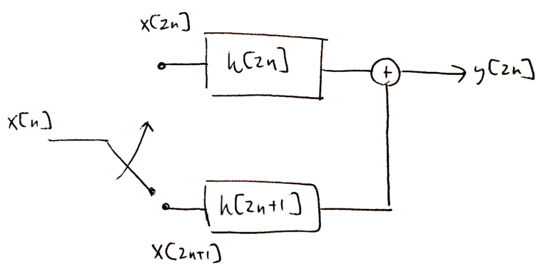
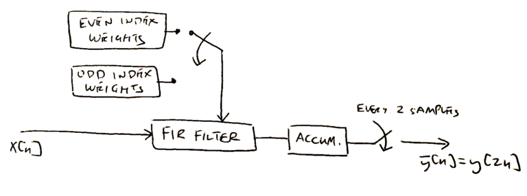
Note from Figure 1 and Figure 2 that the decimation was applied at the output of the LPF where as the decimation is applied at the input of the LPF in Figure 3 . A polyphase filter structure allows each branch of the filter to run at 1/2 the sampling rate which is how it might be implemented in software. Alternatively the polyphase filter structure can be run at the full sampling rate but by doing half of the computation and swapping between the two sets of weights [harris2021, p.194]. Figure 4 demonstrates how the filter weights are swapped into the filtering structure which might be how it is implemented in hardware.

Implementing a Polyphase Filterbank in Software

The HBF weights in Figure 5 will be used to implement a decimate by 2 polyphase filterbank in software. You can find a method to design HBF weights here.

Figure 3 shows that the parallel polyphase filterbank structure has two sub-filters for even and odd indexed weights. It makes writing the software easier (with marginal computational cost) if the two sub-filters are of equal length. Yet the impulse response in Figure 3 is odd-length so it must be zero-padded by 1 sample to make it even length. At first glance it would seem that the zero-padding should occur at the end of the impulse response but is that the correct choice?

Consider that convolution performs a time reversal therefore zero-padding the tail of h[n] with 1 sample will in effect turn add a 1 sample delay to the input which is undesired. Instead a 1 sample zero-pad needs to be added to the beginning of h[n] because the zero-padding ends up being at the end of the time-reversed weights and therefore has no impact on the convolution. The padded h[n] will therefore be $\tilde{h}[n]$ such that

(10) $\begin{equation*}\tilde{h[n]} = h[n-1].\end{equation*}$

The code to zero-pad the impulse response is as follows:

HBFWeightsPad = np.concatenate((np.zeros(1),HBFWeights))

Figure 6 gives the impulse response for h[n] and zero-padded $\tilde{h}[n]$ .

The filter weights $\tilde{h}[n]$ must be partitioned into two branches as in (8) and (9) however the even and odd phrasing will be replaced with filter branch A and B to avoid future confusion. The sub-filter $h_{A}[n]$ and $h_{B}[n]$ are therefore defined as

(11) $\begin{equation*}h_{A}[n] = \tilde{h}[2n],\end{equation*}$

(12) $\begin{equation*}h_{B}[n] = \tilde{h}[2n+1].\end{equation*}$

The code to perform the partioning is given below:

AIndices = np.arange(1,len(HBFWeightsPad),2)
AWeights = HBFWeightsPad[AIndices]
BIndices = np.arange(0,len(HBFWeightsPad),2)
BWeights = HBFWeightsPad[BIndices]

The AIndices variable starts at an index of 1 due to the 1 sample delay of (10). This 1 sample delay turns even indices odd and odd indices even which is incredibly confusing and why the labels A and B are used instead. Example impulse responses of $h_{A}[n]$ and $h_{B}[n]$ are given in Figure 7.

The input x[n] is downampled into $x_{A}[n]$ and $x_{B}[n]$ as in (8) and (9) such that

(13) $\begin{equation*}x_{A}[n] = x[2n],\end{equation*}$

(14) $\begin{equation*}x_{B}[n] = x[2n+1].\end{equation*}$

The code to downsample the input is given by:

xA = x[0::2] xB = x[1::2]

The last step is to put all of the parts together. The polyphase filterbank output is the summation of the convolution of the two branches,

(15) $\begin{equation*}\bar{y}[n] = \left(x_{A}[n] \ast h_{A}[n]\right) + \left(x_{B}[n] \ast h_{B}[n]\right).\end{equation*}$

The code to implement the parallel polyphase filterbank is as follows:

AOutput = np.convolve(AWeights,xA) BOutput = np.convolve(BWeights,xB) yPolyParallel = AOutput + BOutput

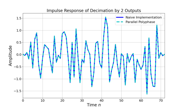
Figure 8 demonstrates the equivalence of the naive decimation from Figure 1 with the polyphase filterbank in Figure 3 by plotting the two outputs after filtering a randomized input signal.

Computational Efficiency

The naive implementation in Figure 1 requires N multiples for each input sample to implement a FIR filter of length N. However the polyphase implementation requires only N multiplies for every 2 input samples, which is 1/2 the work of the naive implementation. Thinking about the performance gain in dB, implementing the decimation saves $1/2 = 10\text{log}_{10}(1/2) = 3~ dB$ which is a great improvement for simply rearranging some filtering.

Additional savings can be obtained through ignoring the zero weights in sub-filter $h_{B}[n]$ as well as folding the even-symmetric weights in sub-filter $h_{A}[n]$ . Both of these filter structures will be covered in a future blog post.

Conclusion

Applying a polyphase filtering structure for decimation by 2 saves 1/2 computation savings as compared to the naive approach. A decimate by 2 HBF is useful in many large sample rate scenarios such as in a Hilbert transformer performing real pass-band to complex baseband conversion or in reducing large sample rates through multiple stages. The implementation can lead to a reduction of multiples in the filter by a factor of 2. Less multiplies means less heat, less cost, smaller hardware and a better overall system.

Have you seen the other posts on the half band filter?

Postscript

P.S. I have worked with polyphase filter banks for over a decade and I still get confused to this day when I try and line up all of the indexing, filter weights, zero-padding and all of the nut and bolts it takes to get them working properly. It usually comes down to getting the code 90% of the way there and just trying a couple of different combinations until it works. Here’s how the conversation in my head usually goes:

Let me try odd index input samples with odd index filter weights, and even with even.
Ok that didn’t work.
Maybe I have an incorrect delay in there somewhere. Let’s try even input samples with odd filter weights.
Ok that didn’t work either.
…
< trying more combinations >
…
Oh I forgot to < insert small overlooked issue >, now it works!

If you are having issues making them work don’t fear, you are not the only one. It took me much longer than I’d like to admit to finish this blog post. Take it step by step and eventually you will get there.