Wave Walker DSP

DSP Algorithms for RF Systems

Buy the Book!

DSP for Beginners: Simple Explanations for Complex Numbers! The second edition includes a new chapter on complex sinusoids.

How to Create Additive White Gaussian Noise (AWGN)

June 1, 2022

Introduction

Creating AWGN is useful in realistic simulations of DSP systems. For example, creating AWGN at proper power levels is useful in simulating bit error rates. If you’re writing a thesis or dissertation on DSP, or you plan to, you’re going to have to generate noise! Read on to find out how to do it correctly.

Check out these other blogs on DSP:

What is Noise?

Noise is what corrupts your signal. Noise is different than interference, which is another signal conflicting with your signal of interest.

However, adding up many types of interference produces Gaussian noise through the central limit theorem. Noise is the addition of all types of interference from cellular radio, AM and FM radio, broadcast TV. Noise also comes from places like the sun and lightning strikes.

Have you ever seen an image of an infrared camera? Physical bodies have a non-zero Kelvin temperature and therefore radiate which is what the infrared camera receives. This also contributes to the noise at your receiver.

The coolest type of noise is cosmic noise. Your radio is even affected by the noise generated from a quasar. I don’t know what that means but it sounds awesome!

Additive White Gaussian Noise (AWGN)

The central limit theorem allows the Gaussian distribution to be used as the model for AWGN. The Gaussian distribution is often referred to as the normal distribution. The noise in this blog is generated, or simulated, using NumPy’s random.normal() function.

Noise Power (or Variance)

The variance of AWGN in the real world will depend on the noise power, however the simplest way to start is to generate complex noise with a variance of 1 and then scale the noise to the desired power.

The variance $\sigma^2$ of the noise $w[n]$ is given by

(1) $\begin{equation*}\sigma^2 = \mathbb{E} \left\{ (w[n] - \mu)(w[n] - \mu)^* \right\}\end{equation*}$

where $\mu$ is the mean of $w[n]$ ,

(2) $\begin{equation*}\mu = \sum_{n=0}^{N-1} w[n].\end{equation*}$

The mean $\mu$ of AWGN is assumed to be zero, therefore the noise variance (or power) in (1) is

(3) $\begin{equation*}\sigma^2 = \mathbb{E} \left\{ w[n] w^*[n] \right\}\end{equation*}$

Creating Real and Imaginary Noise

The time domain of AWGN [proakis2011, p.231] is Gaussian noise for both the real and imaginary components. The noise $w[n]$ is constituted by its real and imaginary components,

(4) $\begin{equation*}w[n] = w_{R}[n] + jw_{I}[n].\end{equation*}$

Substituting (4) into (3),

(5) $\begin{equation*}\begin{split}\sigma^2 & = \mathbb{E} \left\{ \left(w_{R}[n] + jw_{I}[n] \right) \left(w_{R}[n] + jw_{I}[n] \right)^* \right\} \\& = \mathbb{E} \left\{ w_{R}[n]^2 + w_{I}[n]^2 \right\} \\& = \mathbb{E} \left\{ w_{R}[n]^2 \right\} + \mathbb{E} \left\{ w_{I}[n]^2 \right\}.\end{split}\end{equation*}$

The noise power for the real and imaginary terms are therefore

(6) $\begin{equation*}\sigma_{R}^2 = \mathbb{E} \left\{ w_{R}[n]^2 \right\},\end{equation*}$

(7) $\begin{equation*}\sigma_{I}^2 = \mathbb{E} \left\{ w_{I}[n]^2 \right\}.\end{equation*}$

The real and imaginary noise each contribute half of the power to the complex noise power. To generate complex noise with variance 1 then

(8) $\begin{equation*}\sigma_{R}^2 = \frac{1}{2},\end{equation*}$

(9) $\begin{equation*}\sigma_{I}^2 = \frac{1}{2}.\end{equation*}$

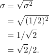
NumPy’s normal.random function requires the standard deviation $\sigma$ of the Gaussian noise, which is

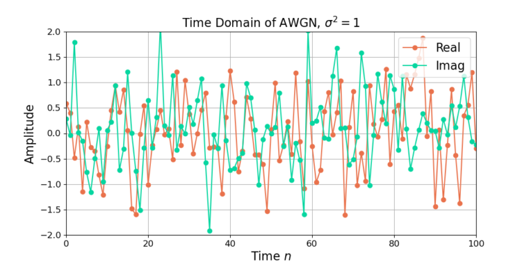
(10) $\begin{equation*}\begin{split}\sigma & = \sqrt{ \sigma^2 }\\& = \sqrt{ (1/2)^2 } \\& = 1/\sqrt{2} \\& = \sqrt{2}/2.\end{split}\end{equation*}$

The noise for both real and imaginary channels is generated by:

noiseReal = np.random.normal(0,np.sqrt(2)/2,numSamples)
noiseImag = np.random.normal(0,np.sqrt(2)/2,numSamples)

which is the combined into the complex signal

noise = noiseReal + 1j*noiseImag

The variance of the complex noise can be checked by:

print(‘noise power = ‘ + str(np.mean(np.abs(noise)**2)))

Scaling the Noise Power

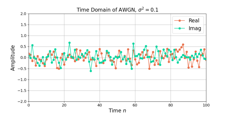
The above Python code creates complex AWGN with a variance (or power) of 1. However, the desired noise power will likely need to be a different value. The noise can be scaled to a different noise power $P_n$ through the equation

(11) $\begin{equation*}w_{scaled}[n] = \sqrt{P_n} w[n]\end{equation*}$

which is implemented in Python by:

noiseScaled = np.sqrt(Pn) * noise

Double-check the scaled noise power in Python:

print(‘scaled noise power = ‘ + str(np.mean(np.abs(noiseScaled)**2)))

Conclusion

Create complex noise by starting with real and imaginary noise with power 0.5 and then adding them together. The result is complex noise with power 1. Then scale the complex noise to the desired power.